Bojie Li
2023-05-27
(This article is organized based on the speech I delivered at Peking University on December 12, 2022, first converting the conference recording into a draft using iFlytek’s speech recognition, then polishing it with GPT-4 to correct errors from voice recognition, and finally manually adding some new thoughts)
I am very grateful to Professor Huang Qun and Professor Xu Chenren for the invitation, and it is an honor to come to Peking University to give a guest lecture for their computer networking course. I heard that you are all the best students at Peking University, and I could only dream of attending Peking University in my days. It is truly an honor to have the opportunity to share with you some of the latest developments in the academic and industrial fields of computer networking today.
Turing Award winner David Patterson gave a very famous speech in 2019 called “A New Golden Age for Computer Architecture”, which talked about the end of Moore’s Law for general-purpose processors and the historic opportunity for the rise of Domain-Specific Architectures (DSA). What I am going to talk about today is that computer networking has also entered a new golden age.

The computer networks we come into contact with daily mainly consist of three parts: wireless networks, wide area networks, and data center networks. They provide the communication foundation for a smart world of interconnected things.
Among them, the terminal devices of wireless networks include mobile phones, PCs, watches, smart homes, smart cars, and various other devices. These devices usually access the network through wireless means (such as Wi-Fi or 5G). After passing through 5G base stations and Wi-Fi hotspots, the devices will enter the wide area network. There are also some CDN servers in the wide area network, which belong to edge data centers. Next, the devices will enter the data center network. In the data center network, there are many different types of devices, such as gateways, servers, etc.

Today, I will introduce you to data center networks, wide area networks, and terminal wireless networks. First, let’s look at data center networks. The biggest change in data center networks is the evolution from simple networks designed for simple web services to networks designed for large-scale heterogeneous parallel computing, performing tasks traditionally handled by supercomputers, such as AI, big data, and high-performance computing.
2023-05-27
** (Article from the WeChat public account of the Intelligent Manufacturing Society, original link, many thanks to the Intelligent Manufacturing Society for their excellent questions and editing) **
What impact will AI ultimately have on the technology and life of human society?
With the release of GPT4, the performance of large model AI has once again refreshed the public’s imagination. The content produced by AIGC is becoming more realistic and refined. With the continuous deepening of data cleaning and training, AI’s understanding of natural language has also shown great progress. From passively accepting data “feeding” to actively asking questions to the world, perhaps, the “artificial intelligence life” in science fiction is no longer far away from us.
Anxiety is inevitable, and “AI unemployment” seems to be really happening in some industries. On May 18, 2023, local time, BT, the largest telecom operator in the UK, said it would cut 40,000 to 55,000 jobs between 2028 and 2030. The layoffs will include BT’s direct employees and third-party employees, reducing the company’s total number of employees by 31-42%. Currently, BT has about 130,000 employees.
BT’s boss Philip Jansen publicly stated that after completing fiber optic deployment, digitizing work methods, adopting artificial intelligence (AI), and simplifying its structure, it will rely on fewer labor and significantly reduced cost base, “the new BT Group will be a leaner enterprise with a brighter future”. Looking back at home, some Internet technology companies have also shown related trends, especially the art outsourcing positions of game companies, which can be described as “disaster areas”.
Speaking of this issue, Li Bojie, assistant scientist at Huawei 2012 Lab, said that some of the public’s anxieties have been magnified by the media. AI technology is not a flood beast that replaces humans, but rather, it liberates productivity and shapes more new jobs. “For example, if we look at the past industrial revolution, people who used to do farming now have to use machines. The education they need, as well as the changes in society, economy, and people’s lifestyle, are all very big.”
Li Bojie believes that after AI technology becomes popular and becomes a new production tool, more industries and occupations will be generated in response. “For example, after the computer, there is no need for a copyist to copy things hard, right? AI is the same, some industries directly involve people, it can’t replace, like the service industry, right? But some things that follow the rules and do fixed patterns, AI can simplify a lot of labor.”
As a researcher of data center network technology closely related to AI, Li Bojie has put forward many views and thoughts on AI. Below is the conversation record of Xiao Zhi, the main writer of the Intelligent Manufacturing Society, and Li Bojie:
2023-05-25
This is an old article of mine from 5 years ago. It was a winter night in early 2018 when I set up a large pot by myself in the Thirteen Tombs and sent a small part of human knowledge to Sirius, 8.6 light-years away. The story behind this can be found here. Today, what we are concerned with is that sending messages to potential extraterrestrial civilizations obviously requires making them recognize that the message is sent by an intelligent life form, and also making them understand it.
A very basic question is, how do you prove your level of intelligence in the message? In other words, if I were an intelligent life form monitoring cosmic signals, how would I determine whether a bunch of signals contains intelligence? Since intelligence is not a matter of having or not having, but rather more or less, how do we measure the degree of intelligence contained in these signals? I think my thoughts from 5 years ago are still interesting, so I’m organizing and posting them.
The message is just a string. Imagine we could intercept all communications from aliens and concatenate them into a long message. How much intelligence does it contain? This is not an easy question to answer.
Current technology generally tries to decode the message and then see if it expresses basic information from sciences such as mathematics, physics, astronomy, logic, etc. The Arecibo message from 1974 was encoded in this way, hoping to attract the attention of extraterrestrial civilizations. I tried to find a purely computational method to measure the level of intelligence contained in the message.
2023-04-20
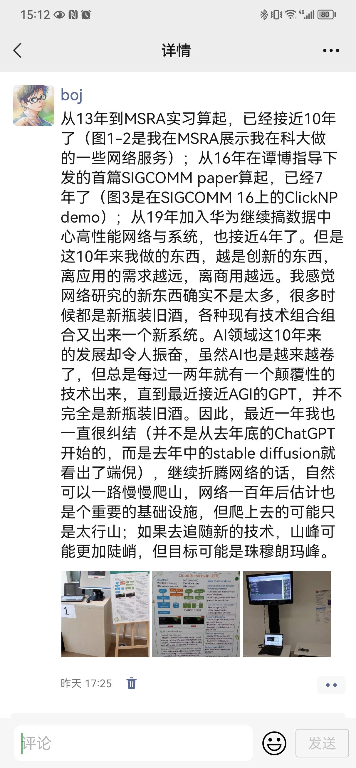
This WeChat Moment from yesterday sparked a lot of discussion both inside and outside the company, and many people reached out to me.
I considered it from two perspectives: innovation and commercialization.
2023-01-29
Long read warning: Part two of the “Five Years of PhD at MSRA” series, about 13,000 words, to be continued…
KV-Direct, published at SOSP 2017, was my second paper (as first author). Since the first SIGCOMM paper ClickNP was done with Bo Tan guiding me step by step, KV-Direct was also the first paper I led on my own.
What to Do After SIGCOMM
After submitting the SIGCOMM paper, Bo Tan said that for the next project, I needed to come up with the direction on my own.
Compiler or Application?
We were well aware that ClickNP still had many issues, with the current support for compilation optimization being too simple. We hoped to enhance the compiler’s reliability from the perspective of programming languages. At the same time, we used ClickNP as a common platform for network research within our group to incubate more research ideas.
Naturally, I explored along two directions, one was to extend ClickNP to make it easier to program and more efficient; the other was to use the ClickNP platform to develop new types of network functions to accelerate various middlewares in the network. At that time, we were exploring many middlewares in parallel, such as encryption/decryption, machine learning, message queues, layer 7 (HTTP) load balancers, key-value stores, all of which could be accelerated with FPGAs.
To improve the programmability of ClickNP, I started looking for good talents from the school to join the MSRA internship. Yi Li was interested in programming languages and formal methods during his undergraduate studies. He was the first student I recommended to intern at MSRA. At the start of the spring semester, Yi Li came to MSRA for his internship, coinciding with the completion of his undergraduate thesis. He proposed several key optimizations for the ClickNP system, added some syntax to simplify programming, and corrected some awkward syntax.
However, due to the workload, we did not do a major overhaul of the compilation framework, still using simple syntax-directed translation without using professional compiler frameworks like clang, nor intermediate languages. Therefore, each time a new compilation optimization was added, it seemed rather ad-hoc.
Encountering various strange issues with OpenCL, I had the idea of creating a high-level synthesis (HLS) tool myself, generating Verilog directly from OpenCL. My idea was simple: for application scenarios in the networking domain, what we do is to unroll all loops in a piece of C code into a large block of combinational logic. By inserting registers at appropriate positions, it could become a pipeline with extremely high throughput, capable of processing an input every clock cycle. If the code accesses global states, then such loop dependencies determine the maximum number of registers on the dependency path, which is the upper limit of the clock frequency.
However, Bo Tan disagreed with my idea of creating an HLS tool ourselves, because we were not professional FPGA researchers. Such work lacked innovation, more about filling the “gaps” of existing HLS tools, a engineering problem, difficult to publish top-tier papers in either FPGA or networking fields.
Due to frequent issues with FPGA card programming, I ended up plugging and unplugging FPGA cards in the server room every day, sometimes debugging on-site. Thus, like my undergraduate days in the minor academy’s server room, I often spent hours in the server room, enduring the cold air and noise over 80 decibels.
2023-01-23
Long article warning: The first in the “Five Years of PhD at MSRA” series, about 12,000 words, to be continued…
On July 31, 2021, at the ACM Turing Conference in China, I was standing on the podium waiting for the ACM China Outstanding Doctoral Dissertation Award. I didn’t expect that the person who came up to present the award to me was President Bao, and my legs involuntarily trembled a bit. This was the only time I had seen President Bao up close. President Bao happily said that seeing one of us from USTC among the award winners shows that USTC can also cultivate masters. He hoped that we could become masters in the future, serve our motherland, and return to our alma mater.
The host of the award ceremony, Professor Liu Yunhao, asked us to talk about the title of our doctoral dissertation and our advisors. I blurted out, “High-Performance Data Center Systems Based on Programmable Network Cards“, my advisors are Professor Chen Enhong from USTC and Dr. Zhang Lintao from Microsoft, and I would like to give special thanks to Dr. Tan Kun from Huawei. I can clearly remember the title of my doctoral dissertation, it’s hanging on my homepage. In the company, people often send me private messages asking if I am the author of a certain paper. I would shyly say, yes…
Many people may think that I am the kind of PhD student who is solely focused on studying, but my PhD life is actually much more interesting than many people imagine, truly embodying the MSRA (Microsoft Research Asia) motto “Work hard, play harder“.
Research Novice
Joint Training
MSRA (Microsoft Research Asia) has joint PhD training programs with many universities in China. Among them, the joint training program with USTC has been ongoing for many years. In the second semester of my junior year, MSRA interviewed dozens of candidates at our school, selected about a dozen students for summer internships and a year-long internship in their senior year, and after the summer internship, about 7 students were confirmed to become joint training PhDs. These joint training PhDs will complete their first year of master’s and doctoral courses at USTC, and the next four years will be spent on academic research at MSRA in Beijing, finally obtaining a PhD degree from USTC.
The requirements for MSRA to select joint training PhDs are the so-called “three good” students: good at math, good at programming, and good attitude. This rule is said to have been set by the former dean, Dr. Shen Xiangyang. Because I spent all day tinkering with various Linux network services in the Youth Class College computer room and LUG activity room during my undergraduate studies, I didn’t study very well, and naturally my grades weren’t very good. My GPA was only 3.4 (out of 4.3), and I even failed Calculus II. The interviewer asked me at the time why my math grades were so poor. Probably because I had won awards in programming competitions (NOI) in high school, and my resume had many network service projects I worked on at LUG, I was surprisingly admitted to the joint training PhD program. The GPAs of other students admitted to the joint training program were at least 3.7, and most of them were top students with 3.8 or above.
2023-01-23
I found a VCD disc from the pile of old papers, which was given to me by Shijiazhuang TV station in 2004. After restoration and transcoding, the interview program “Superstar Li Bojie - Remembering the Hua Luogeng Gold Cup Gold Medalist” broadcasted 19 years ago finally sees the light of day again.
From this 13 and a half minute video, you can see how fat I was back then :) The sports question that was publicly revealed starts at 11:25 in the video :)
2023-01-22

Time: May 1, 2023, 10:58
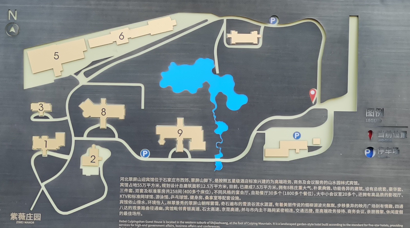
Location: Cui Ping Shan Hotel, Hebei
Transportation Information: Cui Ping Shan Hotel is located at No. 1 Yingbin Road, Luquan District, Shijiazhuang City, Hebei Province.
- As Cui Ping Shan Hotel is located in the western suburbs and is not accessible by subway, public transportation is inconvenient. It is recommended to take a taxi.
- High-speed rail:
- By car: The nearest route from Shijiazhuang High-speed Rail Station is 16 kilometers, and the elevated route is 22 kilometers. It takes about 35 minutes by car without traffic.
- Public transportation: You can take bus 320 / air 320 directly (need to walk 1.3 kilometers), which takes 1 hour and 20 minutes; or take subway line 3 to subway line 1 to tourist bus 5, which takes 1 hour and 10 minutes.
- The taxi queue at Shijiazhuang High-speed Rail Station is very long after 22:00. If you arrive late, it is recommended to contact us in advance for pick-up.
- Airplane:
- By car: It is 53 kilometers from Shijiazhuang Zhengding International Airport, and it takes about 50 minutes by car without traffic.
- Public transportation: From Zhengding Airport, you can take Airport Bus Line 1 (one bus per hour) to Subway Line 1 to Tourist Bus 5, which takes 2 hours and 10 minutes.
- It is inconvenient to take a taxi at Zhengding Airport at night. If you arrive late, it is recommended to contact us in advance for pick-up.
- As the wedding officially begins at 10:58, it is recommended to arrive in Shijiazhuang on April 30. Those departing from Beijing who are short on time can also consider taking the early high-speed rail on May 1 (5 departures from 06:26 to 08:34).

Accommodation Information:
- Try to arrange to stay in Building 6 and Building 9 of Cui Ping Shan Hotel, Hebei, where rooms have been reserved. If there are special circumstances, we will arrange nearby hotels.
- Breakfast is expected to be in Building 6, from 7:00 to 10:00. Bridesmaids, groomsmen, and staff need to leave early and will not have time for breakfast, so a simple meal will be arranged in Buildings 6 and 9.
- The distance between Building 6 and Building 9 is 560 meters, and it takes 8 minutes to walk.
2022-12-13
There’s a classic joke where a student chose a course called “Choices and Future”, only to find out in the classroom that it was about “Options and Futures”, because their English names are both Options and Futures. A few days ago, the hotel where I had a meeting was right across from the Shanghai Futures Exchange, which made me think of a question: What are our judgments and choices about the future based on?
Recently, I read two books, “Gifts Differing” and “How NASA Builds Teams”, and found that this reflects the differences in people’s ways of thinking. Sensing and iNtuition, Thinking and Feeling are the two most critical differences.
Before the main text, you might want to think about the differences in the characters of Sun Wukong, Zhu Bajie, Tang Monk, and Sha Monk in “Journey to the West”, and how they work together as a team?
2022-12-12
Thanks to Professor Xu Chenren and Professor Huang Qun for the invitation, I am very honored to have given a guest lecture for the Computer Network course at Peking University on December 12, 2022.
Abstract: Data center networks, wide area networks, and wireless networks provide the communication cornerstone for the intelligent world of Internet of Things.
Data center networks have traditionally been designed for easily parallelizable web services. But today, AI, big data, HPC are all large-scale heterogeneous parallel computing systems, which have high requirements for communication performance. The heavy software stack causes huge overhead, which requires the communication semantics of data center networks to evolve from byte streams to memory semantics including message semantics, synchronous and asynchronous remote memory access, RPC, and to achieve extreme latency and bandwidth with a combination of software and hardware. In the future, we hope to treat the data center as a computer, on the one hand, to achieve peer-to-peer direct access between heterogeneous computing and storage devices, making the data center interconnection as high-performance as the internal bus of the host; on the other hand, to make distributed system programming as convenient as single-machine programming through Serverless.
Large-scale live streaming and short video on-demand, real-time audio and video communication and other applications pose new challenges to the stability of wide area network transmission. Internet giants have built their own global acceleration networks and designed new transport protocols such as QUIC to achieve a high-quality user experience. In addition, due to the low energy cost in the western part of our country, the strategy of “computing in the east and calculating in the west” has become a national strategy. Through Regionless scheduling, we can achieve a “nationwide integrated large data center”.
Seamless collaboration of intelligent terminals such as mobile phones, PCs, wearable devices, smart homes, smart cars, and industrial Internet applications such as 5G to B all require stable low latency and high bandwidth, which requires wireless protocol stack optimization, and even wireless memory semantics to support Gbps-level bandwidth. In addition, through the “distributed super terminal” programming framework of HarmonyOS, more closely distributed collaboration can be enabled to achieve seamless data and service flow.
Download Slides PDF (Updated on 2022-12-15)
Download Slides PPTX (Updated on 2022-12-15)
Full text of the speech: