Why the Nobel Prize in Physics Was Awarded to AI
(This article was first published in a Zhihu answer to “Why was the 2024 Nobel Prize in Physics awarded to machine learning in artificial neural networks?”)
Some people joked that many physicists hadn’t heard of the two people who won this year’s Nobel Prize in Physics…
The Connection Between Artificial Neural Networks and Statistical Physics Is Not Accidental
In early July, when I returned to my alma mater for the 10th anniversary of my undergraduate graduation, I chatted with some classmates who are into mathematics and physics about AI. I was surprised to find that many fundamental concepts in AI today originate from statistical physics, such as diffusion models and emergence.
@SIY.Z also explained to me the statistical physics foundations behind many classic AI algorithms, such as the significant achievement of the two Nobel laureates, the Restricted Boltzmann Machine (RBM).
This connection is not accidental because statistical physics studies the behavior of systems composed of a large number of particles, just as artificial neural networks are systems composed of a large number of neurons. The early development of artificial neural networks clearly reveals this connection:
Hopfield Network
In 1982, Hopfield, while studying the principles of human memory, aimed to create a mathematical model to explain and simulate how neural networks store and reconstruct information, especially how neurons in the brain form memories through interconnections.
Specifically, the purpose of this research was to construct a CAM (Content-Addressable Memory) that supports “semantic fuzzy matching,” where multiple pieces of data are stored during the storage phase, and during the reconstruction phase, a partially lost or modified piece of data is input to find the original data that matches it best.
The Hopfield network utilized the atomic spin characteristic of matter, which allows each atom to be viewed as a small magnet. This is why the Hopfield network and subsequent artificial neural networks resemble the Ising model in statistical physics, which explains why matter has ferromagnetism.
The overall structure of the network can be described using the energy of spin systems in physics. If energy is imagined as the altitude of the ground and data as the coordinates of north, south, east, and west, a Hopfield network is like a mountainous landscape with many peaks. A small ball dropped from the sky will automatically roll to one of the valleys. The positions of these valleys are the original data that need to be stored.
In the process of storing information, or during training, the connection weights between nodes are determined through layer-by-layer updating rules, so that the stored images correspond to lower energy states. Today, minimizing loss in machine learning training corresponds to the fundamental principle of energy minimization in physics. As the network state is continuously updated, the system’s energy gradually decreases, eventually reaching a local minimum, corresponding to the network’s stable state (attractor). This dynamic process is similar to the process in physical systems that tend toward minimal potential energy.
In the process of reconstructing information, or during inference, when a Hopfield network receives a distorted or incomplete image, it gradually updates the states of nodes to lower the system’s energy, thereby gradually restoring the image most similar to the input.
Hopfield discovered that whether it’s a physical system composed of a large number of particles or a neural network composed of a large number of neurons, they are robust to changes in details; damaging one or two neurons hardly affects the overall characteristics of the system. This makes it possible to incrementally change the weights of a neural network and gradually learn patterns in training data.
The Hopfield network demonstrated that a system composed of a large number of neurons can produce a certain degree of “computational capability” (computational capability is a more academic expression of “intelligence”) and was the first to use simple artificial neurons to replicate the phenomenon of collective emergence in physics.
Although the Hopfield network was a pioneer in artificial neural networks, its network structure was not reasonable (all nodes were fully connected), and the Hebbian learning mechanism was also not reasonable, as the update rules were deterministic rather than randomized, leading to limited learning ability of the Hopfield network, which could only store and reconstruct simple patterns.
This is where Hinton’s Boltzmann machine comes into play.
Boltzmann Machine
In 1983-1985, Hinton and others proposed the Boltzmann machine.
At that time, Hinton and his team’s research goal went further than Hopfield’s, not only studying whether a system composed of a large number of neurons could exhibit memory capabilities but also hoping to simulate the behavior of systems composed of a large number of particles in the physical world. Sora’s idea that “generative models are world simulators” may have originated here. Initially, I thought Sora’s idea came from Ilya Sutskever’s paper, but during the 10th-anniversary reunion with physics classmates, I realized its roots were in the statistical physics of the 1980s.
The Boltzmann machine is also a structure that can store and reconstruct information, but its most important innovation compared to the Hopfield network is already reflected in the word “Boltzmann.”
The Hopfield network assumes that all input data are independent of each other, while the Boltzmann machine assumes that input data follow a certain probability distribution. Therefore, the Boltzmann machine is a probabilistic generative model (yes, the same as the Generative in today’s GPT), which not only tries to reproduce the most similar input data like the Hopfield network but also hopes to simulate the statistical distribution of complex patterns and generate new data similar to the patterns contained in the input data.
Specifically, the Boltzmann machine is based on the maximum likelihood estimation in statistics. Therefore, the Boltzmann machine can extract the structure in data without labeled training data, which is today’s unsupervised learning.
In terms of network structure, update rules, and energy function, the Boltzmann machine also demonstrates the advantages of stochastic models over deterministic models:
Network Structure:
- Hopfield Network: Deterministic model, all nodes are symmetric, and nodes are fully connected.
- Boltzmann Machine: Stochastic model, divides nodes in the neural network into visible and hidden layers, using probability distributions to describe states. The visible layer handles input and output, while the hidden layer is not directly connected to input and output information. However, all nodes are still fully connected.
Update Rules:
- Hopfield Network: Deterministic update rules, node states are updated synchronously or asynchronously, converging to a stable state with minimal energy.
- Boltzmann Machine: The Boltzmann machine simulates the state transition process of the system through sampling (such as Gibbs sampling or other Markov Chain Monte Carlo methods). During sampling, the system gradually converges to a low-energy state. This gradual “cooling” process is similar to the simulated annealing algorithm, which also aims to find the global optimal solution through energy minimization.
Energy Function:
- Hopfield Network: The energy function is deterministic; as the state updates, energy decreases, and the system converges to a local minimum.
- Boltzmann Machine: The energy function defines the system’s probability distribution (i.e., Boltzmann distribution), with low-energy states having higher probabilities. The system finds low-energy states through sampling. This is similar to the “selection” of the optimal path in the principle of least action.
Backpropagation
In 1986, Hinton proposed the backpropagation algorithm, solving the problem of training artificial neural networks and making deep learning possible. Training involves data fitting, using the Boltzmann machine’s fewer parameters to fit the features in a large amount of data, essentially compressing the patterns in training data into the Boltzmann machine. According to Occam’s razor, once training data is compressed, features are extracted, and knowledge is learned.
Restricted Boltzmann Machine
Although the Boltzmann machine is theoretically elegant, it was not very effective in practice. Due to the limited computing power of computers at the time, the fully connected network structure of the Boltzmann machine made convergence difficult. Therefore, in the 1990s, artificial neural networks entered a winter period.
In the early 21st century, Hinton proposed the Restricted Boltzmann Machine (RBM). The most significant innovation of RBM compared to the Boltzmann machine is replacing the fully connected structure with a bipartite graph structure, where only visible nodes and hidden nodes have weights, and there are no weights between nodes of the same type.
Because the Boltzmann machine is fully connected, training is very complex, as it requires handling the interdependencies between all neurons. Especially through Markov Chain Monte Carlo (MCMC) sampling, convergence is slow. However, RBM, due to its restricted bipartite structure (no intra-layer connections), simplifies the training process. The commonly used training method is Contrastive Divergence (CD), which significantly speeds up training and makes RBM more feasible in practical applications. Additionally, the dependencies between the hidden and visible layers are conditionally independent, making the activation of hidden units and weight updates simpler.
The rest of the story is well-known: new activation functions, multi-layer neural networks, skip connections (ResNet), combined with gradually developing computing power, led to the first wave of AI enthusiasm. As for Transformer and GPT, that’s another story after the growth of computing power.
Why the Nobel Prize Was Awarded to AI
Statistical physics, like quantum mechanics, represents a major leap in human understanding of the world. Quantum mechanics is a shift from determinism to probabilism, while statistical physics is a shift from reductionism to system theory.
Before statistical physics, humanity had a reductionist mindset, hoping to attribute the laws of the world’s operation to simple physical laws. But statistical physics made us realize that the characteristics of complex systems are inherently complex and cannot be summarized by a few simple rules. Therefore, to simulate their behavior, we need to use another relatively simple complex system, such as an artificial neural network, to extract their features. Using a relatively simple complex system to simulate a relatively complex complex system is feature recognition and machine learning.
From the Hopfield network to the Boltzmann machine, we see that probabilistic models are the biggest innovation. Modeling the world as a probabilistic model is valid not only for microscopic particles at the quantum mechanics level but also for macroscopic systems composed of a large number of particles.
In fact, Hopfield and Hinton’s initial research goals determined that the Hopfield network would be deterministic, while Hinton would use probabilistic models. Hopfield aimed to memorize and reconstruct existing information, while Hinton aimed to generate information similar to the patterns in existing data. The reason why Hopfield and Hinton won the Nobel Prize this year, rather than during the first wave of AI in 2016, is because the value of generative models has been validated.
Repeating once more, complex systems cannot be explained by simple rules; they need to be modeled using another relatively simple complex system. The behavior of complex systems should be modeled using probabilistic models rather than deterministic ones. These two insights are not obvious. Many people today are still trying to explain the behavior of neural networks with a few simple rules; many believe that deep neural networks are probabilistic models and therefore can never reliably solve mathematical problems. These are misconceptions resulting from a lack of understanding of probability theory.
One of the important goals of physics is to discover the laws governing the operation of the world. The discovery awarded the Nobel Prize in Physics this time is not a specific physical law but a methodology for understanding and simulating complex systems: artificial neural networks. Artificial neural networks are not just applications like cars or computers; they are also a new method for humans to discover the laws of the world. Therefore, although I was surprised by this Nobel Prize in Physics, upon reflection, it makes a lot of sense.
My Personal Bold Opinion
“Generative models are world simulators” This phrase became popular with the advent of Sora, but it was actually proposed by OpenAI as early as 2016, and OpenAI’s chief scientist Ilya Suskever learned this idea from his teacher Hinton.
Thinking carefully about this phrase is quite frightening. The physical world requires a mole-level number of particles to exhibit intelligence. Yet, artificial neural networks can simulate the laws of a mole-level number of particles with several orders of magnitude fewer neurons, exhibiting intelligence. This implies that artificial neural networks are a more efficient form of knowledge representation. In a world with limited energy, artificial neural networks might be a more efficient carrier of intelligence.
We still don’t know where the capability boundaries of artificial neural networks lie. Are they really general enough to model all phenomena in the physical world? The fact is, from Hopfield networks, Boltzmann machines, RBMs, deep neural networks to Transformers, model capabilities are continuously breaking through limitations. Nowadays, some problems considered unsolvable by Transformers are almost being overcome.
For example, mathematical calculations are often considered unsolvable by Transformers, but now CoT (Chain of Thought) and reinforcement learning-based OpenAI o1 have basically solved the problem of large models performing simple numerical and symbolic calculations.
OpenAI o1 can even use world knowledge and logical reasoning abilities to discover some high-level laws from data. For instance, given the first 100 digits of Pi and told that this number has a pattern, it can predict the 101st digit by recognizing it as Pi and accurately calculating it using Pi’s calculation method. Previously, many believed that this knowledge discovery ability and multi-step complex numerical calculations were things Transformers could never handle. There is even a question on Zhihu, “If you feed the first 10 billion digits of π to a large model, will it produce relatively accurate results for the subsequent digits?,” with most answers being sarcastic. But facts have proven that using test-time scaling (increasing inference time for slow thinking), this is indeed possible.
Now, OpenAI o1 mini can solve most undergraduate science course problems, such as the four major mechanics, mathematical analysis, linear algebra, stochastic processes, and differential equations. o1 mini can solve about 70%-80% of complex calculation problems and over 90% of simple concept and calculation problems. Computer science undergraduate coding problems are even less of an issue. I think o1 mini could graduate from undergraduate programs in mathematics, physics, and computer science. The official version of o1 is expected to be even stronger. As I test it, I joke that my own intelligence is limited; I never understood advanced mathematics back then, so I can only use tools smarter than myself to compensate for my intellectual shortcomings.
The ability of humans to discover laws being caught up and surpassed by AI might be a matter of 10 years. Perhaps decades later, the Nobel Prize in Physics will be awarded to AI. At that time, what should we humans do? My thought is that humans should decide the direction of AI. This is what the ousted Ilya Suskever and Jan Leike are doing at OpenAI with Superalignment: ensuring that AI smarter than humans can follow human intentions.
The Nobel Prize website actually explains why the Physics Prize was awarded to Hopfield and Hinton, who work in AI. There are two versions, one more popular and one more in-depth. Both articles are well-written and recommended for reading.
More Popular Nobel Prize Website Introduction
https://www.nobelprize.org/prizes/physics/2024/popular-information/
This year’s laureates used tools from physics to build methods that help lay the foundation for today’s powerful machine learning. John Hopfield created a structure that can store and reconstruct information. Geoffrey Hinton invented a method that can autonomously discover data attributes, which has become very important in the large artificial neural networks used today.
They Used Physics to Find Patterns in Information
Many people have experienced how computers can translate between different languages, interpret images, and even engage in reasonable conversations. Perhaps less known is that this technology has long played an important role in research, including the classification and analysis of massive amounts of data. Over the past fifteen to twenty years, machine learning has advanced rapidly, utilizing a structure known as artificial neural networks. Today, when we talk about artificial intelligence, we usually refer to this technology.
Although computers cannot think, machines can now mimic functions such as memory and learning. This year’s Physics Prize winners helped make all this possible. They used fundamental concepts and methods from physics to develop techniques for processing information using network structures.
Machine learning differs from traditional software, which is more like a recipe. Software receives data, processes it according to a clear description, and generates results, much like someone gathering ingredients and following a recipe to make a cake. In machine learning, computers learn through examples, enabling them to solve problems that are too vague and complex to be handled by step-by-step instructions. An example is interpreting images to identify objects within them.
Mimicking the Brain
Artificial neural networks process information through the entire network structure. The initial inspiration came from understanding how the brain works. As early as the 1940s, researchers began deriving the mathematical principles underlying the network of neurons and synapses in the brain. Another key piece of the puzzle came from psychology, thanks to neuroscientist Donald Hebb’s hypothesis that learning occurs because connections between neurons are strengthened when they work together.
Later, these ideas were used to attempt to recreate the network functions of the brain through computer simulations of artificial neural networks. In these simulations, the brain’s neurons are mimicked by nodes, which are assigned different values, while synapses are represented by connections between nodes that can become stronger or weaker. Hebb’s hypothesis remains one of the basic rules for updating artificial networks through a process called training.
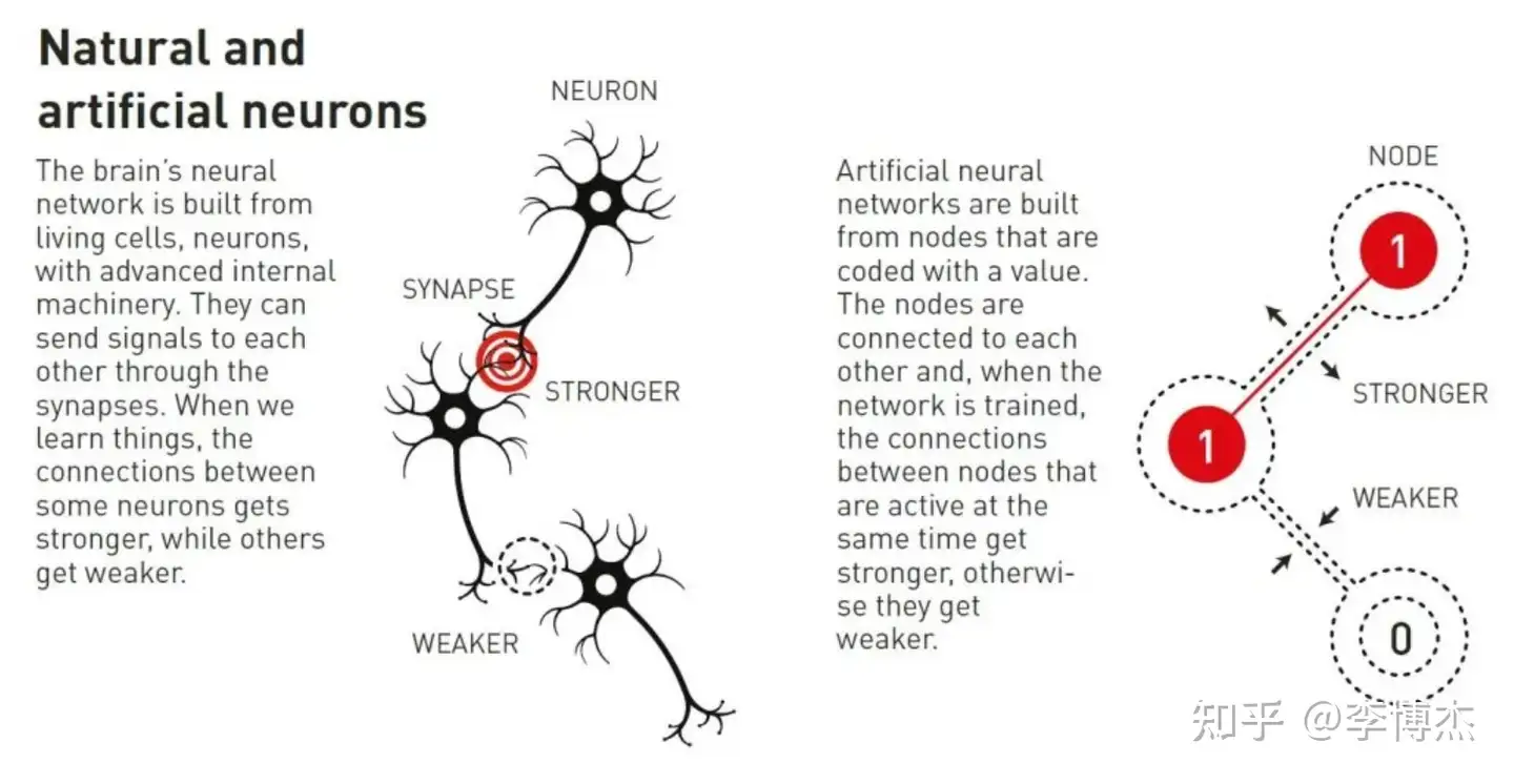 Illustration of natural and artificial neurons
By the late 1960s, some discouraging theoretical results led many researchers to doubt whether these neural networks would have any practical use. However, in the 1980s, several important ideas, including the work of this year’s laureates, reignited interest in artificial neural networks.
Associative Memory
Imagine you are trying to remember a relatively uncommon word that you rarely use, such as the word for the sloped floor usually seen in cinemas or lecture halls. You search through your memory. It’s something like “ramp” (ramp)… maybe “radial” (rad…ial)? No, that’s not it. It’s “rake,” that’s it!
This process of searching for the correct word through similar vocabulary is similar to the associative memory discovered by physicist John Hopfield in 1982. Hopfield networks can store patterns and have a method for reproducing these patterns. When the network receives an incomplete or slightly distorted pattern, this method can find the most similar stored pattern.
Hopfield had previously used his physics background to explore theoretical problems in molecular biology. When he was invited to a conference on neuroscience, he encountered research on brain structures. He was captivated by what he learned and began thinking about the dynamics of simple neural networks. When neurons work together, they can produce new powerful properties that are apparent to those who focus only on the individual components of the network.
In 1980, Hopfield left his position at Princeton University, as his research interests had taken him away from his colleagues in the field of physics, and moved to the continent. He accepted a position as a professor of chemistry and biology at the California Institute of Technology (Caltech), located in Pasadena, Southern California, where he had the freedom to use computer resources for experiments and develop his ideas about neural networks.
However, he did not abandon his foundation in physics, where he found inspiration for understanding how systems composed of many small components can produce new phenomena. He particularly benefited from studying magnetic materials with special properties, where the atomic spins make each atom a tiny magnet. The spins of adjacent atoms influence each other, forming regions with spins in the same direction. He was able to use the physics describing how materials develop when spins interact to construct a model network with nodes and connections.
Networks Store Images in a Landscape
The network Hopfield constructed had nodes interconnected by connections of varying strengths. Each node could store an individual value—in Hopfield’s initial work, this value could be 0 or 1, like pixels in a black-and-white image.
Hopfield described the overall state of the network with a property equivalent to energy in physics; energy is calculated using a formula that takes into account all the node values and the strengths of all the connections between them. The Hopfield network is programmed by inputting images into the nodes, which are assigned values of black (0) or white (1). The connections in the network are then adjusted using the energy formula so that the stored images have lower energy. When another pattern is input into the network, a rule is used to check each node one by one to see if changing the node’s value results in lower energy for the network. If it is found that changing a black pixel to white reduces energy, its color is changed. This process continues until no further improvements can be found. When this point is reached, the network usually reproduces the original image from training.
If you only store one pattern, this might not seem very significant. You might wonder why not just save the image itself and compare it with another image being tested, but the special aspect of Hopfield’s method is that multiple images can be stored simultaneously, and the network can usually distinguish between them.
Hopfield compared the process of a search network preserving states to a ball rolling over a landscape of peaks and valleys, with friction slowing its movement. If the ball is dropped at a certain position, it will roll into the nearest valley and stop there. If a pattern close to a stored pattern is provided to the network, it will proceed in the same way until it reaches the bottom of the energy landscape, thereby finding the closest pattern in its memory.
Hopfield networks can be used to reconstruct data that contains noise or has been partially erased.
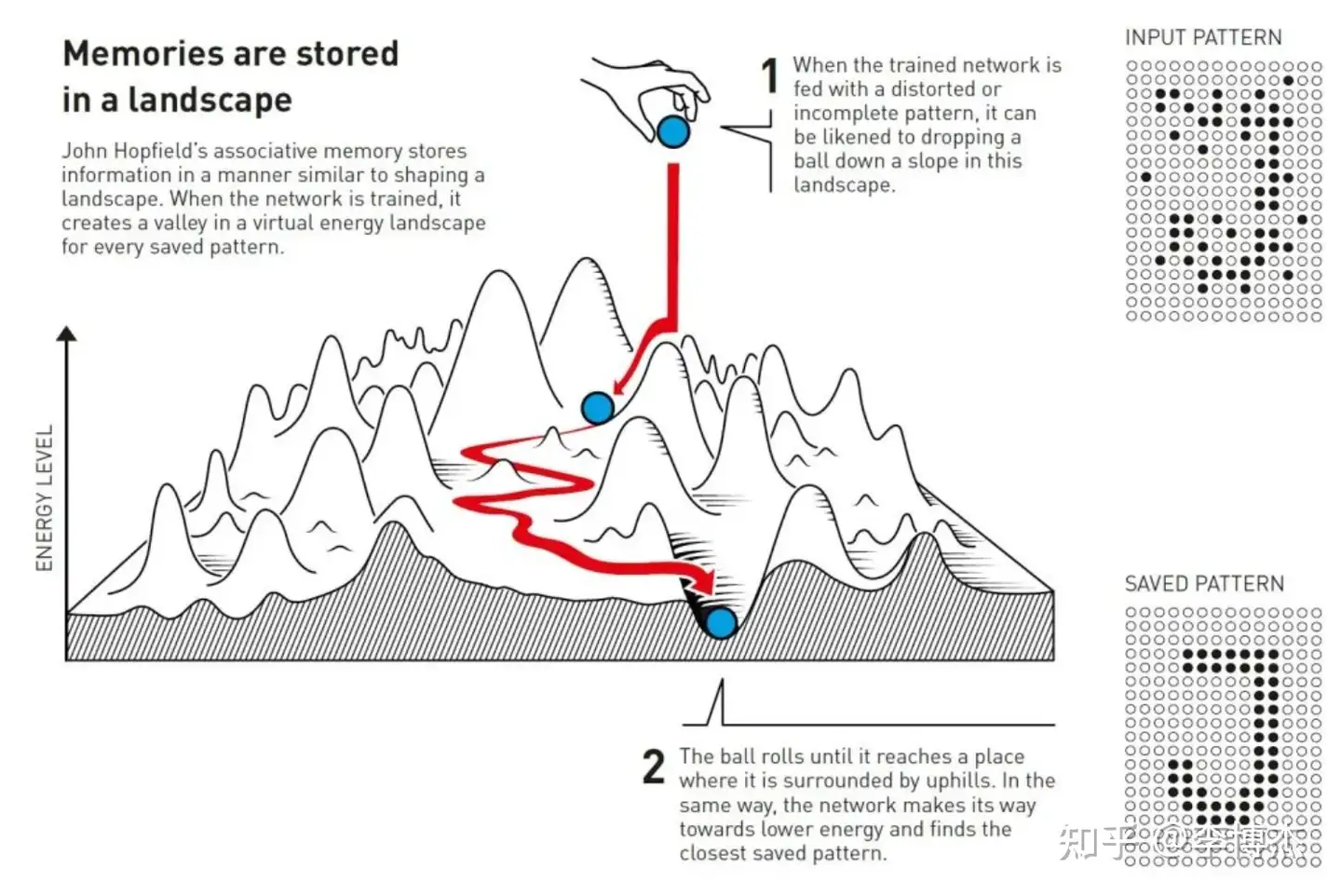 Network preserving images in a landscape
Hopfield and others continued to develop the details of Hopfield networks, including nodes that can store arbitrary values, not just zero or one. If nodes are viewed as pixels in an image, they can have different colors, not just black and white. Improved methods enable the storage of more images, even if they are very similar, and can distinguish between them. It is also possible to recognize or reconstruct any information as long as it is composed of many data points.
Classification Using 19th Century Physics
Remembering an image is one thing, but interpreting what it depicts requires more.
Even very young children can point out different animals and confidently say whether it is a dog, cat, or squirrel. Although they occasionally make mistakes, they quickly become almost always correct. Even without seeing any charts or conceptual explanations about species or mammals, children can learn this. After encountering a few examples of each animal, different categories form in the child’s mind. People learn to recognize cats, understand a word, or enter a room and notice what has changed through experiencing their surroundings.
When Hopfield published his associative memory article, Geoffrey Hinton was working at Carnegie Mellon University in Pittsburgh, USA. He had previously studied experimental psychology and artificial intelligence in England and Scotland and was pondering whether machines could learn to process patterns like humans, finding their own classification methods to organize and interpret information. Together with his colleague Terrence Sejnowski, Hinton started from Hopfield networks and constructed new models using ideas from statistical physics.
Statistical physics describes systems composed of many similar elements, such as molecules in a gas.
While it is difficult to track all the molecules in a gas, the overall properties of the gas, such as pressure or temperature, can be determined through the whole. There are many ways gas molecules can diffuse at individual speeds within their volume, but the same collective attributes can still be derived.
Statistical physics can analyze the states in which components coexist and calculate the probabilities of their occurrence. Some states are more likely to occur than others; this depends on the system’s energy, described by equations from 19th-century physicist Ludwig Boltzmann. Hinton’s network utilized this equation, and the method was published in 1985 under the catchy name “Boltzmann Machine.”
Recognizing New Instances of the Same Kind
Boltzmann machines typically use two different types of nodes. Information is input into a set called visible nodes. Another set of nodes forms a hidden layer. The values and connections of hidden nodes also affect the energy of the entire network.
Boltzmann machines operate by rules that update node values one by one. Eventually, the machine will reach a state where the pattern of nodes can change, but the overall properties of the network remain unchanged. Each possible pattern has a specific probability, depending on the network energy calculated according to the Boltzmann equation. When the machine stops, it generates a new pattern, making the Boltzmann machine an early generative model.
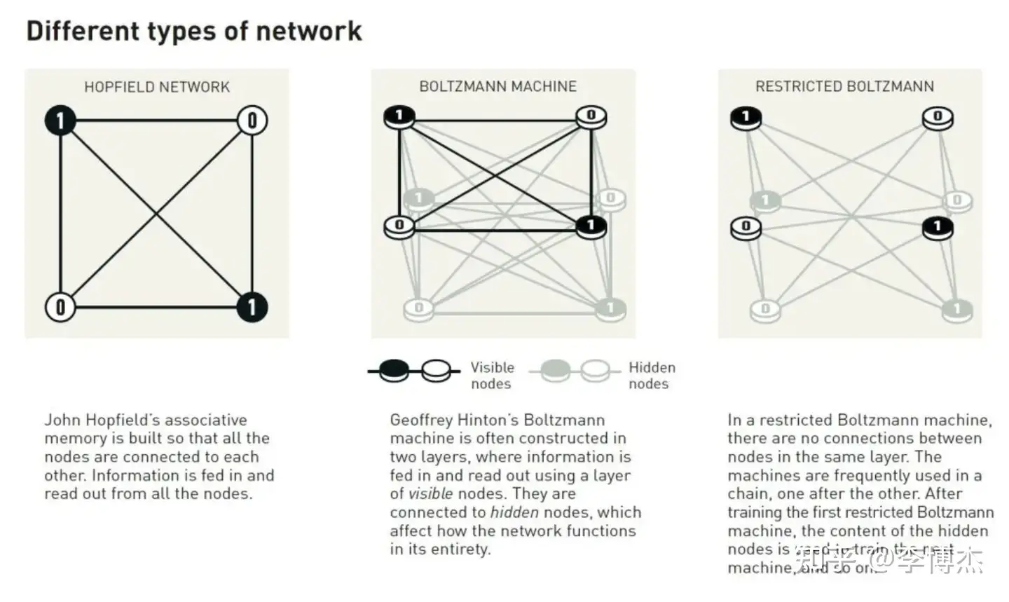 Different types of neural networks
Boltzmann machines learn through examples—not through instructions but through examples provided to them. Its training process involves updating the values in the network connections to maximize the probability of occurrence of example patterns input to the visible nodes during training. If the same pattern is repeated multiple times during training, its probability will be higher. Training also affects the probability of generating new patterns similar to the training examples.
A trained Boltzmann machine can recognize familiar features in information it has never seen before. Imagine meeting a friend’s sibling and immediately recognizing that they must be related. In a similar way, a Boltzmann machine can recognize entirely new instances belonging to categories in the training material and distinguish them from materials of different categories.
In its original form, the Boltzmann machine was inefficient, taking a long time to find solutions. When it was developed in different ways, things became more interesting, and Hinton continued to explore this. Later versions were simplified by removing some connections between units. It turned out that this could make the machine more efficient.
In the 1990s, many researchers lost interest in artificial neural networks, but Hinton was one of the few scholars who continued to work in this field. He also helped initiate a new wave of exciting results; in 2006, he and colleagues Simon Osindero, Yee Whye Teh, and Ruslan Salakhutdinov developed a method for pre-training networks, pre-training layer by layer in multiple Boltzmann machine hierarchies. This pre-training provided a better starting point for the connections in the network, optimizing its training to recognize elements in images.
Boltzmann machines are often used as part of larger networks. For example, they can recommend movies or TV shows based on viewer preferences.
Machine Learning—Today and Tomorrow
We owe thanks to the work that began in the 1980s, with John Hopfield and Geoffrey Hinton helping lay the foundation for the machine learning revolution that began around 2010.
The development we are witnessing now is due to the availability of large amounts of data for training networks and the significant increase in computing power. Today’s artificial neural networks are often large and composed of multiple layers. These are called deep neural networks, and their training method is known as deep learning.
A quick look at Hopfield’s 1982 article on associative memory can give us an understanding of this development. In the article, he used a network with 30 nodes. If all nodes are connected to each other, there would be 435 connections. Nodes have their own values, and connections have different strengths, with less than 500 parameters to track in total. He also tried a network with 100 nodes, but it was too complex for the computers used at the time to handle. We can compare this to today’s large language models, which consist of networks built with hundreds of millions of parameters.
Now, many researchers are developing applications for machine learning. Which applications will become the most promising remains to be seen, while extensive ethical discussions are also unfolding around the development and use of this technology.
Since physics provided tools for the development of machine learning, it is noteworthy that physics as a research field has also benefited greatly from artificial neural networks. Machine learning has long been used in fields familiar from previous Nobel Prizes in Physics. These fields include the use of massive data processing to discover the Higgs boson; another application includes reducing noise in measurements of gravitational waves from colliding black holes or searching for exoplanets.
In recent years, this technology has also begun to be used to calculate and predict the properties of molecules and materials—for example, calculating the structure of protein molecules that determine their function or studying which versions of new materials might have the most suitable properties for more efficient solar cells.
A deeper introduction on the Nobel Prize website
https://www.nobelprize.org/uploads/2024/09/advanced-physicsprize2024.pdf
“Foundational Discoveries and Inventions Inspired by Artificial Neural Networks for Machine Learning”
The 2024 Nobel Prize in Physics is awarded by the Royal Swedish Academy of Sciences to John Hopfield and Geoffrey Hinton for their foundational contributions to artificial neural networks (ANN) and their advancement of the field of machine learning.
Introduction
Since the 1940s, machine learning based on artificial neural networks (ANNs) has developed into a versatile and powerful tool over the past three decades, applicable in both everyday life and cutting-edge scientific fields. Through artificial neural networks, the boundaries of physics have been extended to the phenomena of life and the field of computation.
Artificial neural networks, inspired by biological neurons in the brain, contain a large number of “neurons” or nodes that interact through “synapses” or weighted connections. They are trained to perform specific tasks rather than execute a predetermined set of instructions. Their basic structure closely resembles spin models applied in statistical physics to theories of magnetism or alloys. This year’s Nobel Prize in Physics recognizes the breakthrough methodological advances in the field of artificial neural networks achieved by leveraging this connection.
Historical Background
In the 1940s, the first electronic-based computers emerged, initially invented for military and scientific purposes, designed to perform tedious and time-consuming calculations for humans. By the 1950s, there was a reverse demand to have computers perform pattern recognition tasks that humans and other mammals excel at.
This attempt to achieve artificial intelligence was initially initiated by mathematicians and computer scientists who developed programs based on logical rules. This approach continued until the 1980s, but the computational resources required for precise classification of images, among other things, became too expensive.
Meanwhile, researchers began exploring how biological systems solve pattern recognition problems. As early as 1943, neuroscientist Warren McCulloch and logician Walter Pitts proposed a model of how neurons in the brain collaborate. In their model, neurons form a weighted sum of binary input signals from other neurons, which determines a binary output signal. Their work became the starting point for later research on biological and artificial neural networks.
In 1949, psychologist Donald Hebb proposed a mechanism for learning and memory, where the simultaneous and repeated activation of two neurons leads to the strengthening of the synapse between them.
In the field of artificial neural networks, two architectures of node interconnection systems were explored: “recurrent networks” and “feedforward networks.” The former allows feedback interactions, while the latter contains input and output layers, possibly with hidden layers sandwiched in between.
In 1957, Frank Rosenblatt proposed a feedforward network for image interpretation and implemented this network in computer hardware. The network contained three layers of nodes, with only the weights between the middle layer and the output layer being adjustable, and these weights were determined in a systematic manner.
Rosenblatt’s system attracted considerable attention but had limitations in handling nonlinear problems. A simple example is the “either one or the other, but not both” XOR problem. Marvin Minsky and Seymour Papert pointed out these limitations in their 1969 book, leading to a funding stagnation in artificial neural network research.
During this period, parallel developments inspired by magnetic systems aimed to create models for recurrent neural networks and study their collective properties.
Progress in the 1980s
In the 1980s, significant breakthroughs were made in the fields of recurrent neural networks and feedforward neural networks, leading to a rapid expansion in the field of artificial neural networks.
John Hopfield was a prominent figure in the field of biophysics. His pioneering work in the 1970s studied electron transfer between biomolecules and error correction in biochemical reactions (known as kinetic proofreading).
In 1982, Hopfield published an associative memory model based on a simple recurrent neural network. Collective phenomena frequently occur in physical systems, such as domain structures in magnetic systems and vortices in fluids. Hopfield proposed whether “computational” capabilities might emerge in the collective phenomena of a large number of neurons.
He noted that the collective properties of many physical systems are robust to changes in model details, and he explored this issue using a neural network with N binary nodes sis_is_i (0 or 1). The network’s dynamics are asynchronous, with individual nodes undergoing threshold updates at random times. The new value of node sis_is_i is determined by the weighted sum of all other nodes:
h\_i = \\sum\_{j \\neq i} w\_{ij} s\_j
If h\_i > 0, then s\_i = 1, otherwise s\_i = 0 (with the threshold set to zero). The connection weights w\_{ij} are considered to reflect the correlation between node pairs in stored memories, known as the Hebb rule. The symmetry of the weights ensures the stability of the dynamics. Static states are identified as non-local memories stored on the N nodes. Additionally, the network is assigned an energy function E:
E = - \\sum\_{i < j} w\_{ij} s\_i s\_j
During the network’s dynamics, the energy monotonically decreases. Notably, as early as the 1980s, the connection between physics and artificial neural networks became apparent through these two equations. The first equation can be used to represent the Weiss molecular field (proposed by French physicist Pierre Weiss), describing the arrangement of atomic magnetic moments in solids, while the second equation is commonly used to evaluate the energy of magnetic configurations, such as ferromagnets. Hopfield was well aware of the application of these equations in describing magnetic materials.
Metaphorically, the dynamics of this system drive the N nodes to the bottom of an N-dimensional energy landscape, corresponding to the system’s static states. Static states represent memories learned through the Hebb rule. Initially, the number of memories that could be stored in Hopfield’s dynamic model was limited. Methods to alleviate this issue were developed in later work.
Hopfield used his model as associative memory and as a tool for error correction or pattern completion. A system with an erroneous pattern (e.g., a misspelled word) would be attracted to the nearest local energy minimum for correction. The model gained more attention when it was discovered that the fundamental properties of the model, such as storage capacity, could be analyzed using methods from spin glass theory.
A reasonable question at the time was whether the properties of this model were a product of its coarse binary structure. Hopfield answered this question by creating a simulated version of the model with continuous-time dynamics given by the equations of motion of electronic circuits. His analysis of the simulated model showed that binary nodes could be replaced with analog nodes without losing the collective properties of the original model. The static states of the simulated model correspond to the mean-field solutions of the binary system at an effectively adjustable temperature and approach the static states of the binary model at low temperatures.
Hopfield and David Tank utilized the continuous-time dynamics of the simulated model to develop a method for solving complex discrete optimization problems. They chose to use the dynamics of the simulated model to obtain a “softer” energy landscape, facilitating the search. Optimization was performed by gradually reducing the effective temperature of the simulated system, analogous to the simulated annealing process in global optimization. This method solves optimization problems by integrating the equations of motion of electronic circuits, during which nodes do not require instructions from a central unit. The method is one of the pioneering examples of using dynamical systems to solve complex discrete optimization problems, with more recent examples being quantum annealing.
By creating and exploring these physics-based dynamical models, Hopfield made foundational contributions to our understanding of the computational capabilities of neural networks.
Boltzmann Machines
Between 1983 and 1985, Geoffrey Hinton, along with Terrence Sejnowski and other colleagues, developed a stochastic extension of Hopfield’s 1982 model, known as the Boltzmann machine. Each state s = (s\_1, ..., s\_N) in a Boltzmann machine is assigned a probability following a Boltzmann distribution:
P(s) \\propto e^{-E/T}, E = - \\sum\_{i < j} w\_{ij} s\_i s\_j - \\sum\_{i} \\theta\_i s\_i
where T is a fictitious temperature, and \\theta\_i is a bias or local field.
The Boltzmann machine is a generative model, unlike the Hopfield model, which focuses on the statistical distribution of patterns rather than a single pattern. It includes visible nodes corresponding to the patterns to be learned, as well as hidden nodes introduced to model more general probability distributions.
The weights and bias parameters of the Boltzmann machine define the energy E, and these parameters are determined through training to minimize the deviation between the statistical distribution of visible patterns generated by the model and the statistical distribution of given training patterns. Hinton and his colleagues developed an elegantly formal gradient-based learning algorithm to determine these parameters. However, each step of the algorithm involves time-consuming equilibrium simulations for two different sets.
Although theoretically interesting, the practical application of Boltzmann machines was relatively limited in the early stages. However, a simplified version, known as the Restricted Boltzmann Machine (RBM), evolved into a versatile tool (see the next section).
Both the Hopfield model and Boltzmann machines are recurrent neural networks. The 1980s also witnessed significant advances in feedforward networks. In 1986, David Rumelhart, Hinton, and Ronald Williams demonstrated how to train architectures with one or more hidden layers for classification using an algorithm called backpropagation. The goal here is to minimize the mean square deviation D between the network output and the training data through gradient descent. This requires calculating the partial derivatives of D with respect to all weights in the network. Rumelhart, Hinton, and Williams reinvented a scheme that had been applied by other researchers to related problems. Moreover, more importantly, they demonstrated that networks with hidden layers could be trained using this method to perform tasks known to be unsolvable by networks without hidden layers. They also elucidated the function of hidden nodes.
Moving Towards Deep Learning
The methodological breakthroughs of the 1980s quickly led to successful applications, including pattern recognition in images, language, and clinical data. An important approach was the multilayer convolutional neural network (CNN), trained using backpropagation by Yann LeCun and Yoshua Bengio. The CNN architecture originated from the neocognitron method created by Kunihiko Fukushima, inspired by the work of David Hubel and Torsten Wiesel, who won the Nobel Prize in Physiology or Medicine in 1981. The CNN method developed by LeCun and his colleagues began to be used by American banks in the mid-1990s to classify handwritten digits on checks. Another successful example is the long short-term memory (LSTM) method invented by Sepp Hochreiter and Jürgen Schmidhuber in the 1990s, a recurrent network for processing sequential data, such as speech and language, which can be mapped to a multilayer network through time unfolding.
Despite the successful applications of some multilayer architectures in the 1990s, training deep networks with densely connected layers remained a challenge. For many researchers in the field, training dense multilayer networks seemed out of reach. This situation changed in the 2000s. Hinton was a leader in this breakthrough, with RBM being an important tool.
RBM networks have weights only between visible and hidden nodes, with no weights between nodes of the same type. For RBMs, Hinton created an efficient approximate learning algorithm called contrastive divergence, which is much faster than the algorithm for full Boltzmann machines. Subsequently, he, along with Simon Osindero and Yee-Whye Teh, developed a method for layer-by-layer pre-training of multilayer networks, with each layer trained using an RBM. An early application of this method was autoencoder networks for dimensionality reduction. After pre-training, global parameter fine-tuning can be performed using the backpropagation algorithm. Through RBM pre-training, structures in the data, such as corners in images, can be extracted without labeled training data. Once these structures are identified, labeling through backpropagation becomes relatively simple.
By connecting pre-trained layers in this way, Hinton successfully achieved examples of deep and dense networks, marking a milestone towards today’s deep learning. Later, other methods could replace RBM pre-training to achieve the same performance of deep and dense artificial neural networks.
Artificial Neural Networks as Powerful Tools in Physics and Other Scientific Fields
The previous sections mainly discussed how physics has driven the invention and development of artificial neural networks. Conversely, artificial neural networks are increasingly becoming powerful tools for modeling and analysis in physics.
In some applications, artificial neural networks are used as function approximators, meaning they are used to provide a “replica” of the physical model being studied. This can significantly reduce the required computational resources, allowing for the study of larger systems at higher resolutions. Significant progress has been made in this way, such as in the quantum mechanics many-body problem. Deep learning architectures are trained to reproduce the energy of phases of materials and the shape and strength of interatomic forces, achieving accuracy comparable to ab initio quantum mechanical models. Through these atomistic models trained by artificial neural networks, the phase stability and dynamic properties of new materials can be determined more quickly. Examples of successful applications of these methods include predicting new photovoltaic materials.
These models can also be used to study phase transitions and the thermodynamic properties of water. Similarly, the development of artificial neural network representations has made it possible to achieve higher resolutions in explicit physical climate models without requiring additional computational power.
Applications of Artificial Neural Networks in Particle Physics and Astronomy
In the 1990s, artificial neural networks (ANNs) became standard data analysis tools in increasingly complex particle physics experiments. For example, extremely rare fundamental particles like the Higgs boson exist only briefly in high-energy collisions (e.g., the Higgs boson’s lifetime is about 10−2210^{-22}10^{-22} seconds). The existence of these particles needs to be inferred from track information and energy deposits in detectors. Typically, the expected detector signals are very rare and may be mimicked by more common background processes. To identify particle decays and improve analysis efficiency, artificial neural networks are trained to pick out specific patterns from large amounts of rapidly generated detector data.
Artificial neural networks improved the sensitivity of Higgs boson searches at the Large Electron-Positron Collider (LEP) at CERN in the 1990s and played a role in the analysis that led to the discovery of the Higgs boson at CERN’s Large Hadron Collider (LHC) in 2012. Artificial neural networks were also used in top quark studies at Fermilab.
In astrophysics and astronomy, artificial neural networks have also become standard data analysis tools. A recent example is the neural network-driven analysis using data from the Antarctic IceCube neutrino detector, which generated a neutrino image of the Milky Way. The Kepler mission used artificial neural networks to identify transiting exoplanets. The Event Horizon Telescope image of the black hole at the center of the Milky Way also used artificial neural networks for data processing.
So far, the most significant scientific breakthrough achieved using deep learning artificial neural network methods is the development of the AlphaFold tool, which can predict the three-dimensional structure of proteins based on amino acid sequences. In industrial physics and chemical modeling, artificial neural networks are also playing an increasingly important role.
Applications of Artificial Neural Networks in Daily Life
The list of daily applications based on artificial neural networks is very long. These networks support almost everything we do on computers, such as image recognition, language generation, and more.
Decision support in healthcare is also a mature application of artificial neural networks. For example, a recent prospective randomized study showed that using machine learning to analyze mammograms significantly improved breast cancer detection rates. Another recent example is motion correction technology for magnetic resonance imaging (MRI) scans.
Conclusion
The pioneering methods and concepts developed by Hopfield and Hinton have played a key role in shaping the field of artificial neural networks. Additionally, Hinton has been instrumental in advancing deep and dense artificial neural network methods.
Their breakthroughs, built on the foundations of physical sciences, have shown us a new way to use computers to help solve many of the challenges facing society. Simply put, thanks to their work, humanity now has a new tool that can be used for good purposes. Machine learning based on artificial neural networks is revolutionizing science, engineering, and daily life. The field is already paving the way for breakthroughs in building a sustainable society, such as helping to identify new functional materials. The future use of deep learning and artificial neural networks depends on how we humans choose to use these powerful tools that already play an important role in our lives.